Consider The Following Probability Distribution

four.two Probability Distributions for Discrete Random Variables

Learning Objectives

1. To acquire the concept of the probability distribution of a discrete random variable.
2. To learn the concepts of the mean, variance, and standard deviation of a discrete random variable, and how to compute them.

Probability Distributions

Associated to each possible value x of a detached random variable X is the probability $P\left(x\right)$ that Ten will have the value x in one trial of the experiment.

Definition

The probability distributionA list of each possible value and its probability. of a discrete random variable 10 is a list of each possible value of X together with the probability that X takes that value in one trial of the experiment.

The probabilities in the probability distribution of a random variable Ten must satisfy the following two conditions:

1. Each probability $P\left(x\right)$ must be between 0 and 1: $0\le P\left(\mathrm{ten}\right)\le \mathrm{one}.$
2. The sum of all the probabilities is 1: ${\displaystyle \mathrm{\Sigma }P\left(\mathrm{10}\right)=1}.$

Example 1

A off-white coin is tossed twice. Let X be the number of heads that are observed.

1. Construct the probability distribution of X.
2. Find the probability that at least i head is observed.

Solution:

1. The possible values that X can take are 0, 1, and 2. Each of these numbers corresponds to an event in the sample space $\mathrm{Due\; south}=\left\{hh,ht,th,tt\right\}$ of equally likely outcomes for this experiment: Ten = 0 to $\left\{tt\right\}$ , X = ane to $\left\{ht,th\right\}$ , and X = 2 to $\left\{hh\right\}.$ The probability of each of these events, hence of the corresponding value of Ten, tin can exist plant just past counting, to give

   $$\begin{array}{cccc}x& 0& 1& \mathrm{two}\\ P\left(\mathrm{ten}\right)& 0.25& \mathrm{0.fifty}& 0.25\end{array}$$

   This table is the probability distribution of Ten.

2. "At to the lowest degree one head" is the event Ten ≥ 1, which is the union of the mutually exclusive events X = i and X = 2. Thus

   $$P\left(X\ge 1\right)=P\left(1\right)+P\left(2\right)=\mathrm{0.l}+0.25=0.75$$

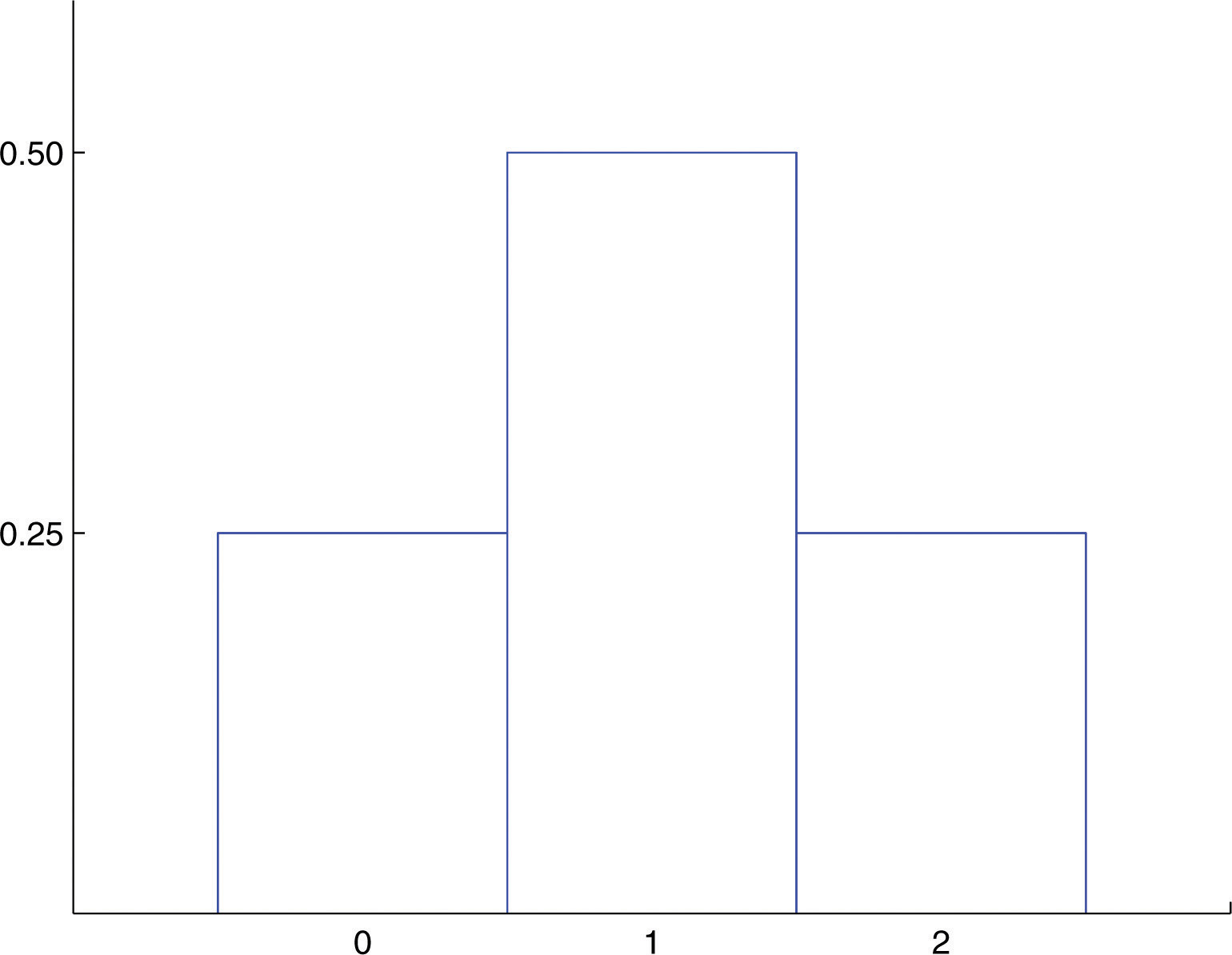
   A histogram that graphically illustrates the probability distribution is given in Figure 4.i "Probability Distribution for Tossing a Fair Coin Twice".

Figure four.1 Probability Distribution for Tossing a Fair Money Twice

Instance 2

A pair of off-white dice is rolled. Permit X denote the sum of the number of dots on the top faces.

1. Construct the probability distribution of 10.
2. Observe P(10 ≥ 9).
3. Find the probability that Ten takes an even value.

Solution:

The sample space of every bit likely outcomes is

$$\begin{array}{cccccc}\mathrm{xi}& 12& \mathrm{xiii}& 14& 15& 16\\ 21& 22& 23& 24& 25& 26\\ 31& 32& 33& 34& 35& 36\\ 41& 42& 43& 44& 45& 46\\ 51& 52& 53& 54& 55& 56\\ 61& 62& 63& 64& 65& 66\end{array}$$

1. The possible values for X are the numbers 2 through 12. X = 2 is the event {11}, then $P\left(2\right)=1∕36.$ 10 = 3 is the event {12,21}, then $P\left(3\right)=2∕36.$ Continuing this way we obtain the table

   $$\begin{array}{cccccccccccc}x& 2& 3& \mathrm{four}& 5& 6& \mathrm{seven}& 8& \mathrm{ix}& 10& 11& 12\\ P\left(x\right)& \frac{\mathrm{i}}{36}& \frac{2}{36}& \frac{\mathrm{iii}}{36}& \frac{\mathrm{four}}{36}& \frac{5}{36}& \frac{6}{36}& \frac{5}{36}& \frac{4}{36}& \frac{\mathrm{iii}}{36}& \frac{2}{36}& \frac{\mathrm{ane}}{36}\end{array}$$

   This table is the probability distribution of X.

2. The upshot Ten ≥ 9 is the wedlock of the mutually sectional events X = ix, X = 10, X = 11, and Ten = 12. Thus

   $$P\left(\mathrm{Ten}\ge \mathrm{nine}\right)=P\left(9\right)+P\left(10\right)+P\left(\mathrm{eleven}\right)+P\left(12\right)=\frac{4}{36}+\frac{\mathrm{iii}}{36}+\frac{\mathrm{ii}}{36}+\frac{1}{36}=\frac{10}{36}=0.2\stackrel{-}{7}$$

3. Before we immediately leap to the conclusion that the probability that X takes an even value must be 0.5, notation that 10 takes half dozen different fifty-fifty values merely simply five unlike odd values. We compute

   $$\begin{array}{lll}\hfill P\left(X\text{\hspace{0.17em}is\hspace{0.17em}even}\right)& =& P\left(2\right)+P\left(\mathrm{iv}\right)+P\left(6\right)+P\left(8\right)+P\left(\mathrm{ten}\right)+P\left(12\right)\\ & =& \frac{1}{36}+\frac{\mathrm{three}}{36}+\frac{\mathrm{five}}{36}+\frac{5}{36}+\frac{3}{36}+\frac{\mathrm{ane}}{36}=\frac{18}{36}=0.5\end{array}$$

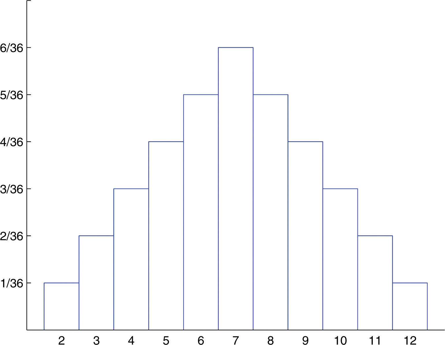
   A histogram that graphically illustrates the probability distribution is given in Figure 4.2 "Probability Distribution for Tossing Two Fair Dice".

Effigy 4.2 Probability Distribution for Tossing Ii Off-white Dice

The Hateful and Standard Deviation of a Detached Random Variable

Definition

The meanThe number ${\displaystyle \mathrm{\Sigma }xP\left(x\right)}$ , measuring its average upon repeated trials. (besides chosen the expected valueIts mean. ) of a discrete random variable Ten is the number

$$\mathit{\mu }=E\left(X\right)=\mathrm{\Sigma }xP\left(x\right)$$

The hateful of a random variable may be interpreted every bit the average of the values assumed by the random variable in repeated trials of the experiment.

Example iii

Detect the mean of the discrete random variable X whose probability distribution is

$$\begin{array}{ccccc}x& \text{−}\mathrm{ii}& \mathrm{ane}& 2& \mathrm{three.5}\\ P\left(x\right)& 0.21& 0.34& 0.24& 0.21\end{array}$$

Solution:

The formula in the definition gives

$$\begin{array}{lll}\hfill \mathit{\mu }& =& \mathrm{\Sigma }xP\left(x\right)\\ & =& \left(\text{−}2\right)·0.21+\left(1\right)·0.34+\left(\mathrm{two}\right)·0.24+\left(\mathrm{iii.5}\right)·0.21=1.135\end{array}$$

Instance 4

A service system in a large boondocks organizes a raffle each month. One 1000 raffle tickets are sold for $one each. Each has an equal chance of winning. First prize is $300, 2d prize is $200, and 3rd prize is $100. Allow 10 denote the net proceeds from the purchase of one ticket.

1. Construct the probability distribution of X.
2. Find the probability of winning any money in the purchase of ane ticket.
3. Find the expected value of 10, and interpret its significant.

Solution:

1. If a ticket is selected every bit the first prize winner, the cyberspace gain to the purchaser is the $300 prize less the $i that was paid for the ticket, hence X = 300 − i = 299. There is one such ticket, so P(299) = 0.001. Applying the same "income minus outgo" principle to the second and third prize winners and to the 997 losing tickets yields the probability distribution:

   $$\begin{array}{ccccc}x& 299& 199& 99& \text{−}1\\ P\left(x\right)& 0.001& 0.001& 0.001& 0.997\end{array}$$

2. Allow W denote the result that a ticket is selected to win i of the prizes. Using the table

   $$P\left(W\right)=P\left(299\right)+P\left(199\right)+P\left(99\right)=0.001+0.001+0.001=0.003$$

3. Using the formula in the definition of expected value,

   $$E\left(X\right)=299·0.001+199·0.001+99·0.001+\left(\text{−}1\right)·0.997=\text{−}0.4$$

   The negative value ways that one loses money on the average. In particular, if someone were to purchase tickets repeatedly, then although he would win now so, on average he would lose xl cents per ticket purchased.

The concept of expected value is too basic to the insurance industry, as the post-obit simplified example illustrates.

Instance 5

A life insurance company will sell a $200,000 i-year term life insurance policy to an private in a particular risk grouping for a premium of $195. Find the expected value to the company of a single policy if a person in this risk group has a 99.97% chance of surviving 1 year.

Solution:

Let X denote the cyberspace gain to the visitor from the sale of 1 such policy. At that place are two possibilities: the insured person lives the whole year or the insured person dies before the year is upwardly. Applying the "income minus outgo" principle, in the former case the value of X is 195 − 0; in the latter case it is $195-\mathrm{200,000}=\text{−}\mathrm{199,805}.$ Since the probability in the first case is 0.9997 and in the second case is $1-0.9997=0.0003$ , the probability distribution for X is:

$$\begin{array}{ccc}x& 195& \text{−}\mathrm{199,805}\\ P\left(\mathrm{ten}\right)& 0.9997& 0.0003\end{array}$$

Therefore

$$E\left(\mathrm{10}\right)=\mathrm{\Sigma }xP\left(x\right)=195·0.9997+\left(\text{−}\mathrm{199,805}\right)·0.0003=135$$

Occasionally (in fact, 3 times in ten,000) the company loses a big amount of money on a policy, but typically it gains $195, which by our computation of $E\left(X\right)$ works out to a internet gain of $135 per policy sold, on average.

Definition

The variance, ${\mathit{\sigma }}^2$ , of a discrete random variable X is the number

$${\mathit{\sigma }}^{\mathrm{ii}}=\mathrm{\Sigma }{\left(x-\mathit{\mu }\right)}^{2}P\left(x\right)$$

which past algebra is equivalent to the formula

$${\mathit{\sigma }}^2=\left[\right.\mathrm{\Sigma }{\mathrm{ten}}^{2}P\left(x\right)\left]\right.-{\mathit{\mu }}^2$$

Definition

The standard differenceThe number $\sqrt{{\displaystyle \mathrm{\Sigma }{(\mathrm{10}-\mathit{\mu })}^{2}P\left(\mathrm{ten}\right)}}$ (also computed using $\sqrt{\left[{\displaystyle \mathrm{\Sigma }{x}^{2}P\left(x\right)}\right]-{\mathit{\mu }}^2}$ ), measuring its variability under repeated trials. , σ, of a discrete random variable X is the foursquare root of its variance, hence is given by the formulas

$$\mathit{\sigma }=\sqrt{\mathrm{\Sigma }{\left(x-\mathit{\mu }\right)}^{\mathrm{ii}}P\left(x\right)}=\sqrt{\left[\right.\mathrm{\Sigma }{x}^{\mathrm{ii}}P\left(\mathrm{ten}\right)\left]\right.-{\mathit{\mu }}^2}$$

The variance and standard deviation of a discrete random variable X may be interpreted as measures of the variability of the values causeless by the random variable in repeated trials of the experiment. The units on the standard deviation match those of X.

Instance six

A discrete random variable X has the post-obit probability distribution:

$$\begin{array}{ccccc}x& \text{−}\mathrm{one}& 0& \mathrm{one}& 4\\ P\left(x\right)& 0.2& \mathrm{0.five}& a& \mathrm{0.ane}\end{array}$$

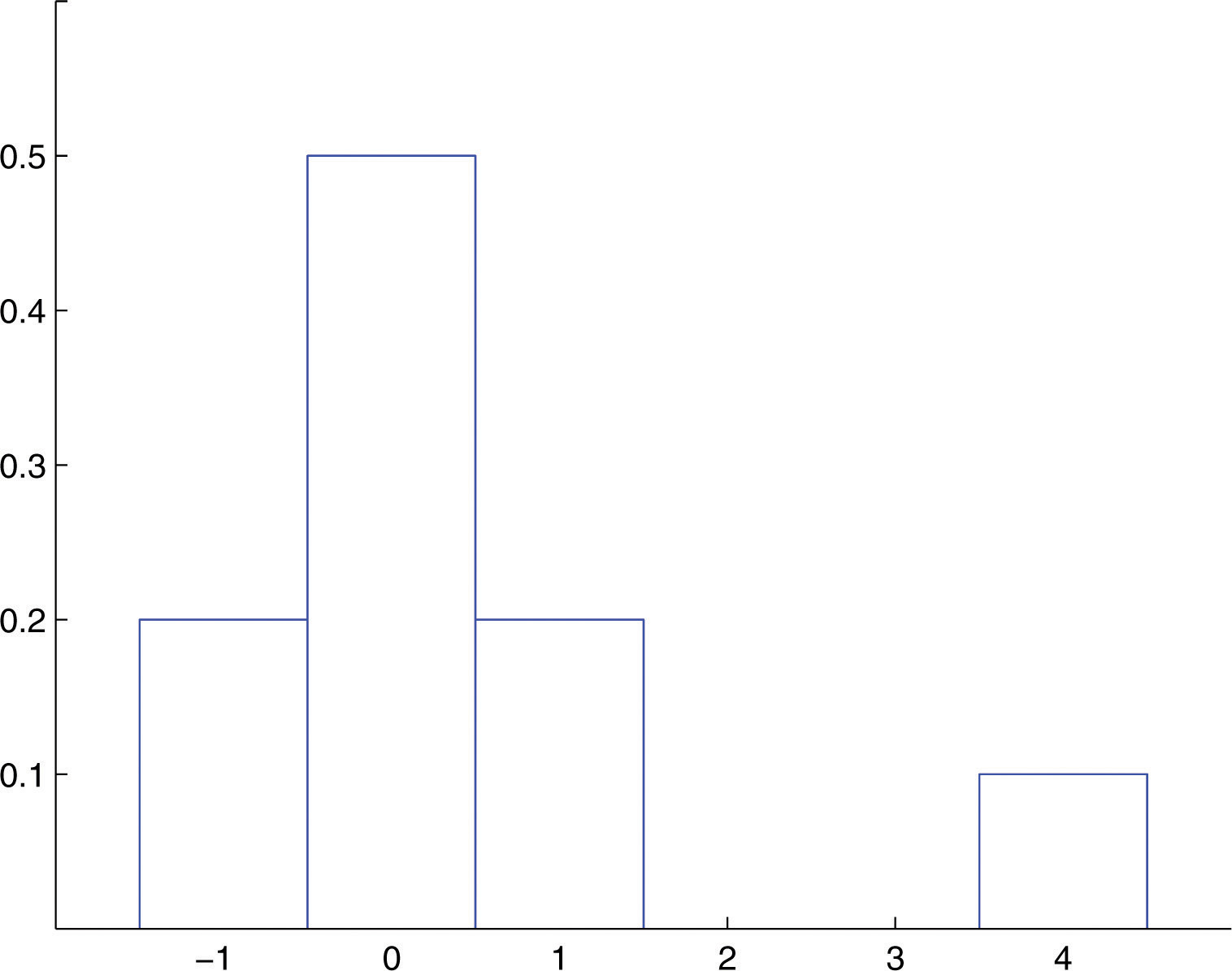
A histogram that graphically illustrates the probability distribution is given in Effigy four.three "Probability Distribution of a Discrete Random Variable".

Figure 4.3 Probability Distribution of a Detached Random Variable

Compute each of the following quantities.

1. a.
2. $P\left(0\right).$
3. P(X > 0).
4. P(X ≥ 0).
5. $P\left(\mathrm{10}\le \text{−}2\right).$
6. The mean μ of X.
7. The variance ${\mathit{\sigma }}^2$ of X.
8. The standard deviation σ of X.

Solution:

1. Since all probabilities must add together upward to 1, $a=1-\left(\mathrm{0.ii}+\mathrm{0.five}+\mathrm{0.i}\right)=\mathrm{0.two}.$
2. Direct from the table, $P\left(0\right)=0.5.$
3. From the table, $P\left(\mathrm{10}>0\right)=P\left(1\right)+P\left(4\right)=0.2+0.1=0.3.$
4. From the table, $P\left(X\ge 0\right)=P\left(0\right)+P\left(1\right)+P\left(\mathrm{iv}\right)=\mathrm{0.five}+0.2+\mathrm{0.ane}=\mathrm{0.eight}.$
5. Since none of the numbers listed as possible values for Ten is less than or equal to −2, the event 10 ≤ −2 is impossible, so P(Ten ≤ −2) = 0.

6. Using the formula in the definition of μ,

   $$\mathit{\mu }=\mathrm{\Sigma }xP\left(\mathrm{10}\right)=\left(\text{−}\mathrm{i}\right)·0.2+0·0.5+\mathrm{i}·\mathrm{0.ii}+4·0.1=0.4$$

7. Using the formula in the definition of ${\mathit{\sigma }}^{\mathrm{two}}$ and the value of μ that was just computed,

   $$\begin{array}{lll}\hfill {\mathit{\sigma }}^2& =& \mathrm{\Sigma }{\left(x-\mathit{\mu }\right)}^{2}P\left(\mathrm{10}\right)\\ & =& {\left(\text{−}1-\mathrm{0.four}\right)}^2·0.2+{\left(0-\mathrm{0.iv}\right)}^2·0.5+{\left(1-0.4\right)}^2·0.2+{\left(4-0.4\right)}^{\mathrm{two}}·0.1\\ & =& 1.84\end{array}$$
8. Using the outcome of part (g), $\mathit{\sigma }=\sqrt{1.84}=1.3565.$

Key Takeaways

• The probability distribution of a discrete random variable X is a listing of each possible value x taken by Ten along with the probability $P\left(x\right)$ that X takes that value in one trial of the experiment.
• The mean μ of a discrete random variable 10 is a number that indicates the average value of X over numerous trials of the experiment. It is computed using the formula $\mathit{\mu }={\displaystyle \mathrm{\Sigma }xP\left(x\right)}.$
• The variance ${\mathit{\sigma }}^{\mathrm{ii}}$ and standard departure σ of a discrete random variable X are numbers that indicate the variability of X over numerous trials of the experiment. They may exist computed using the formula ${\mathit{\sigma }}^2=\left[{\displaystyle \mathrm{\Sigma }{x}^{\mathrm{ii}}}P\left(x\right)\right]-{\mathit{\mu }}^{\mathrm{two}}$ , taking the square root to obtain σ.

Exercises

Basic

1. Determine whether or non the tabular array is a valid probability distribution of a discrete random variable. Explain fully.

   1. $\begin{array}{ccccc}x& \text{−}\mathrm{ii}& 0& 2& 4\\ P\left(x\right)& 0.3& \mathrm{0.five}& \mathrm{0.two}& 0.1\end{array}$

   2. $\begin{array}{cccc}x& \mathrm{0.v}& 0.25& 0.25\\ P\left(x\right)& \text{−}0.4& 0.6& 0.8\end{array}$

   3. $\begin{array}{cccccc}\mathrm{ten}& 1.1& \mathrm{2.v}& \mathrm{iv.1}& \mathrm{4.six}& 5.3\\ P\left(\mathrm{ten}\right)& 0.16& 0.14& \mathrm{0.xi}& 0.27& 0.22\end{array}$

2. Make up one's mind whether or non the table is a valid probability distribution of a detached random variable. Explain fully.

   1. $\begin{array}{cccccc}\mathrm{ten}& 0& 1& 2& 3& 4\\ P\left(x\right)& \text{−}0.25& \mathrm{0.l}& 0.35& 0.10& 0.30\end{array}$

   2. $\begin{array}{cccc}x& 1& 2& 3\\ P\left(x\right)& 0.325& 0.406& 0.164\end{array}$

   3. $\begin{array}{cccccc}x& 25& 26& 27& 28& 29\\ P\left(x\right)& 0.13& 0.27& 0.28& \mathrm{0.eighteen}& 0.14\end{array}$

3. A discrete random variable X has the following probability distribution:

   $$\begin{array}{cccccc}\mathrm{ten}& 77& 78& 79& \mathrm{fourscore}& 81\\ P\left(x\right)& \mathrm{0.xv}& 0.15& 0.20& 0.40& 0.10\end{array}$$

   Compute each of the following quantities.

   1. $P\left(80\right).$
   2. P(X > lxxx).
   3. P(X ≤ lxxx).
   4. The hateful μ of X.
   5. The variance ${\mathit{\sigma }}^{\mathrm{ii}}$ of X.
   6. The standard deviation σ of Ten.

4. A discrete random variable X has the following probability distribution:

   $$\begin{array}{cccccc}x& 13& 18& \mathrm{twenty}& 24& 27\\ P\left(x\right)& 0.22& 0.25& 0.20& 0.17& 0.16\end{array}$$

   Compute each of the following quantities.

   1. $P\left(18\right).$
   2. P(X > xviii).
   3. P(X ≤ 18).
   4. The mean μ of 10.
   5. The variance ${\mathit{\sigma }}^{\mathrm{two}}$ of 10.
   6. The standard deviation σ of 10.

5. If each die in a pair is "loaded" so that one comes up half equally often as information technology should, half dozen comes upwards half again every bit often as it should, and the probabilities of the other faces are unaltered, then the probability distribution for the sum X of the number of dots on the top faces when the two are rolled is

   $$\begin{array}{ccccccc}x& 2& \mathrm{iii}& 4& 5& 6& \mathrm{seven}\\ P\left(x\right)& \frac{1}{144}& \frac{4}{144}& \frac{8}{144}& \frac{12}{144}& \frac{16}{144}& \frac{22}{144}\end{array}$$ $$\begin{array}{cccccc}x& \mathrm{viii}& \mathrm{ix}& \mathrm{ten}& 11& 12\\ P\left(x\right)& \frac{24}{144}& \frac{20}{144}& \frac{16}{144}& \frac{12}{144}& \frac{9}{144}\end{array}$$

   Compute each of the following.

   1. $P\left(5\le X\le 9\right).$
   2. P(X ≥ 7).
   3. The hateful μ of 10. (For off-white dice this number is 7.)
   4. The standard deviation σ of X. (For fair die this number is about 2.415.)

Applications

6. Borachio works in an automotive tire factory. The number Ten of audio but blemished tires that he produces on a random day has the probability distribution

   $$\begin{array}{ccccc}x& 2& 3& 4& \mathrm{five}\\ P\left(\mathrm{ten}\right)& 0.48& 0.36& 0.12& 0.04\end{array}$$

   1. Find the probability that Borachio will produce more than three blemished tires tomorrow.
   2. Detect the probability that Borachio volition produce at most ii blemished tires tomorrow.
   3. Compute the mean and standard deviation of X. Interpret the mean in the context of the problem.

7. In a hamster breeder's feel the number 10 of live pups in a litter of a female person not over twelve months in age who has not borne a litter in the past vi weeks has the probability distribution

   $$\begin{array}{cccccccc}x& 3& 4& \mathrm{five}& \mathrm{six}& 7& 8& 9\\ P\left(\mathrm{10}\right)& 0.04& 0.10& 0.26& 0.31& 0.22& 0.05& 0.02\end{array}$$

   1. Discover the probability that the next litter will produce five to vii live pups.
   2. Notice the probability that the next litter will produce at least half-dozen live pups.
   3. Compute the mean and standard deviation of 10. Interpret the mean in the context of the problem.

8. The number X of days in the summer months that a structure coiffure cannot piece of work because of the weather has the probability distribution

   $$\begin{array}{cccccc}x& 6& \mathrm{seven}& 8& 9& \mathrm{ten}\\ P\left(\mathrm{ten}\right)& 0.03& 0.08& 0.15& 0.20& 0.19\end{array}$$ $$\begin{array}{ccccc}x& 11& 12& 13& 14\\ P\left(x\right)& \mathrm{0.sixteen}& \mathrm{0.ten}& 0.07& 0.02\end{array}$$

   1. Notice the probability that no more than ten days volition be lost next summertime.
   2. Find the probability that from 8 to 12 days will exist lost adjacent summer.
   3. Find the probability that no days at all will be lost side by side summer.
   4. Compute the mean and standard departure of 10. Translate the hateful in the context of the problem.

9. Allow X announce the number of boys in a randomly selected three-child family. Assuming that boys and girls are as likely, construct the probability distribution of Ten.

10. Let X denote the number of times a fair coin lands heads in three tosses. Construct the probability distribution of X.

11. 5 yard lottery tickets are sold for $1 each. 1 ticket will win $1,000, two tickets volition win $500 each, and ten tickets will win $100 each. Let X denote the net gain from the purchase of a randomly selected ticket.

    1. Construct the probability distribution of X.
    2. Compute the expected value $E\left(\mathrm{10}\right)$ of X. Interpret its meaning.
    3. Compute the standard deviation σ of X.

12. Seven grand lottery tickets are sold for $5 each. Ane ticket will win $2,000, two tickets will win $750 each, and five tickets will win $100 each. Allow X denote the net proceeds from the purchase of a randomly selected ticket.

    1. Construct the probability distribution of Ten.
    2. Compute the expected value $E\left(X\right)$ of X. Interpret its significant.
    3. Compute the standard deviation σ of X.

13. An insurance company will sell a $xc,000 one-twelvemonth term life insurance policy to an private in a particular risk grouping for a premium of $478. Find the expected value to the company of a unmarried policy if a person in this hazard group has a 99.62% chance of surviving one year.

14. An insurance company will sell a $10,000 one-year term life insurance policy to an individual in a item gamble grouping for a premium of $368. Find the expected value to the visitor of a single policy if a person in this risk group has a 97.25% adventure of surviving one year.

15. An insurance company estimates that the probability that an private in a particular risk grouping will survive ane year is 0.9825. Such a person wishes to buy a $150,000 ane-year term life insurance policy. Let C denote how much the insurance company charges such a person for such a policy.

    1. Construct the probability distribution of X. (Two entries in the table will contain C.)
    2. Compute the expected value $E\left(X\right)$ of X.
    3. Determine the value C must have in gild for the visitor to break even on all such policies (that is, to average a internet gain of zero per policy on such policies).
    4. Determine the value C must have in order for the company to average a net gain of $250 per policy on all such policies.

16. An insurance company estimates that the probability that an private in a particular risk grouping volition survive 1 year is 0.99. Such a person wishes to buy a $75,000 one-year term life insurance policy. Let C denote how much the insurance company charges such a person for such a policy.

    1. Construct the probability distribution of X. (Two entries in the table will comprise C.)
    2. Compute the expected value $\mathrm{Eastward}\left(\mathrm{10}\right)$ of X.
    3. Determine the value C must have in lodge for the company to intermission even on all such policies (that is, to average a net gain of cipher per policy on such policies).
    4. Decide the value C must have in order for the visitor to average a internet gain of $150 per policy on all such policies.

17. A roulette bike has 38 slots. Thirty-half-dozen slots are numbered from 1 to 36; one-half of them are crimson and half are black. The remaining two slots are numbered 0 and 00 and are green. In a $1 bet on ruby-red, the bettor pays $1 to play. If the ball lands in a reddish slot, he receives dorsum the dollar he bet plus an additional dollar. If the ball does not state on red he loses his dollar. Allow X denote the net gain to the bettor on one play of the game.

    1. Construct the probability distribution of X.
    2. Compute the expected value $\mathrm{Eastward}\left(X\right)$ of 10, and interpret its meaning in the context of the problem.
    3. Compute the standard deviation of X.

18. A roulette bicycle has 38 slots. Xxx-six slots are numbered from 1 to 36; the remaining two slots are numbered 0 and 00. Suppose the "number" 00 is considered not to exist even, only the number 0 is still even. In a $ane bet on fifty-fifty, the bettor pays $one to play. If the brawl lands in an fifty-fifty numbered slot, he receives back the dollar he bet plus an additional dollar. If the ball does not land on an even numbered slot, he loses his dollar. Allow 10 announce the net gain to the bettor on 1 play of the game.

    1. Construct the probability distribution of X.
    2. Compute the expected value $\mathrm{East}\left(X\right)$ of X, and explain why this game is not offered in a casino (where 0 is not considered even).
    3. Compute the standard deviation of X.

19. The time, to the nearest whole infinitesimal, that a metropolis coach takes to get from one terminate of its route to the other has the probability distribution shown. As sometimes happens with probabilities computed as empirical relative frequencies, probabilities in the table add up only to a value other than one.00 because of round-off error.

    $$\begin{array}{ccccccc}x& 42& 43& 44& 45& 46& 47\\ P\left(x\right)& \mathrm{0.x}& 0.23& 0.34& 0.25& 0.05& 0.02\end{array}$$

    1. Observe the average fourth dimension the bus takes to drive the length of its road.
    2. Detect the standard deviation of the length of time the autobus takes to drive the length of its road.

20. Tybalt receives in the mail service an offer to enter a national sweepstakes. The prizes and chances of winning are listed in the offering as: $5 meg, one chance in 65 million; $150,000, one chance in vi.5 million; $5,000, one risk in 650,000; and $1,000, one chance in 65,000. If it costs Tybalt 44 cents to mail his entry, what is the expected value of the sweepstakes to him?

Additional Exercises

21. The number X of nails in a randomly selected ane-pound box has the probability distribution shown. Find the average number of nails per pound.

    $$\begin{array}{cccc}x& 100& 101& 102\\ P\left(\mathrm{10}\right)& 0.01& 0.96& 0.03\end{array}$$

22. Iii fair dice are rolled at once. Let 10 announce the number of die that land with the same number of dots on acme as at least one other die. The probability distribution for Ten is

    $$\begin{array}{cccc}x& 0& u& \mathrm{three}\\ P\left(x\right)& p& \frac{\mathrm{fifteen}}{36}& \frac{1}{36}\end{array}$$

    1. Find the missing value u of 10.
    2. Notice the missing probability p.
    3. Compute the mean of X.
    4. Compute the standard deviation of X.

23. 2 fair dice are rolled at once. Let X denote the difference in the number of dots that announced on the meridian faces of the ii dice. Thus for instance if a one and a five are rolled, X = 4, and if two sixes are rolled, X = 0.

    1. Construct the probability distribution for X.
    2. Compute the mean μ of X.
    3. Compute the standard deviation σ of 10.

24. A fair coin is tossed repeatedly until either information technology lands heads or a total of five tosses have been made, whichever comes get-go. Let X denote the number of tosses fabricated.

    1. Construct the probability distribution for X.
    2. Compute the hateful μ of 10.
    3. Compute the standard deviation σ of X.

25. A manufacturer receives a certain component from a supplier in shipments of 100 units. Two units in each shipment are selected at random and tested. If either one of the units is lacking the shipment is rejected. Suppose a shipment has 5 defective units.

    1. Construct the probability distribution for the number X of defective units in such a sample. (A tree diagram is helpful.)
    2. Find the probability that such a shipment will be accepted.

26. Shylock enters a local branch banking concern at 4:xxx p.1000. every payday, at which time there are ever two tellers on duty. The number 10 of customers in the bank who are either at a teller window or are waiting in a single line for the next available teller has the following probability distribution.

    $$\begin{array}{ccccc}x& 0& 1& 2& \mathrm{iii}\\ P\left(\mathrm{ten}\right)& 0.135& 0.192& 0.284& 0.230\end{array}$$ $$\begin{array}{cccc}\mathrm{ten}& 4& 5& 6\\ P\left(x\right)& 0.103& 0.051& 0.005\end{array}$$

    1. What number of customers does Shylock near often see in the banking concern the moment he enters?
    2. What number of customers waiting in line does Shylock most oftentimes see the moment he enters?
    3. What is the boilerplate number of customers who are waiting in line the moment Shylock enters?

27. The possessor of a proposed outdoor theater must determine whether to include a cover that volition allow shows to be performed in all weather weather condition. Based on projected audience sizes and conditions weather condition, the probability distribution for the revenue X per nighttime if the embrace is not installed is

    $$\begin{array}{lll}\text{Weather}\hfill & \hfill x\hfill & \hfill P\left(x\right)\hfill \\ \text{Clear}\hfill & \hfill \text{\$3000}\hfill & \hfill \text{0}\text{.61}\hfill \\ \text{Threatening}\hfill & \hfill \text{\$2800}\hfill & \hfill \text{0}\text{.17}\hfill \\ \text{Light\hspace{0.17em}rain}\hfill & \hfill \text{\$1975}\hfill & \hfill \text{0}\text{.11}\hfill \\ \text{Show-cancelling\hspace{0.17em}pelting}\hfill & \hfill \text{\$0}\hfill & \hfill \text{0}\text{.eleven}\hfill \end{array}$$

    The boosted cost of the cover is $410,000. The owner will take information technology built if this cost tin can be recovered from the increased acquirement the cover affords in the commencement ten 90-night seasons.

    1. Compute the hateful revenue per night if the comprehend is not installed.
    2. Use the answer to (a) to compute the projected total acquirement per 90-night flavour if the cover is not installed.
    3. Compute the projected total acquirement per season when the cover is in place. To do so presume that if the cover were in identify the revenue each night of the season would be the aforementioned as the revenue on a articulate nighttime.
    4. Using the answers to (b) and (c), decide whether or non the additional cost of the installation of the cover will exist recovered from the increased revenue over the first ten years. Will the possessor accept the cover installed?

Answers

1. 1. no: the sum of the probabilities exceeds one
   2. no: a negative probability
   3. no: the sum of the probabilities is less than 1
3. 1. 0.4
   2. 0.1
   3. 0.9
   4. 79.15
   5. ${\mathit{\sigma }}^2=1.5275$
   6. σ = 1.2359
5. 1. 0.6528
   2. 0.7153
   3. μ = 7.8333
   4. ${\mathit{\sigma }}^2=5.4866$
   5. σ = 2.3424

7. 1. 0.79
   2. 0.60
   3. μ = 5.eight, σ = 1.2570

11. 1. $\begin{array}{ccccc}\mathrm{ten}& \text{−}\mathrm{ane}& 999& 499& 99\\ P\left(\mathrm{10}\right)& \frac{4987}{5000}& \frac{1}{5000}& \frac{\mathrm{two}}{5000}& \frac{10}{5000}\end{array}$

    2. −0.four
    3. 17.8785

13. 136

15. 1. $\begin{array}{ccc}\mathrm{ten}& C& C\text{−}\mathrm{150,000}\\ P\left(\mathrm{ten}\right)& 0.9825& 0.0175\end{array}$

    2. $C\text{−}2625$
    3. C ≥ 2625
    4. C ≥ 2875

17. 1. $\begin{array}{ccc}x& \text{−}\mathrm{one}& 1\\ P\left(x\right)& \frac{20}{38}& \frac{18}{38}\end{array}$

    2. $E\left(X\right)=\text{−}0.0526$ In many bets the bettor sustains an average loss of about 5.25 cents per bet.
    3. 0.9986
19. 1. 43.54
    2. 1.2046

21. 101.02

23. 1. $\begin{array}{ccccccc}\mathrm{10}& 0& 1& 2& \mathrm{three}& 4& 5\\ P\left(x\right)& \frac{6}{36}& \frac{10}{36}& \frac{\mathrm{viii}}{36}& \frac{\mathrm{half-dozen}}{36}& \frac{4}{36}& \frac{2}{36}\end{array}$

    2. i.9444
    3. 1.4326

25. 1. $\begin{array}{cccc}\mathrm{ten}& 0& \mathrm{one}& 2\\ P\left(x\right)& 0.902& 0.096& 0.002\end{array}$

    2. 0.902
27. 1. 2523.25
    2. 227,092.5
    3. 270,000
    4. The owner will install the cover.

Consider The Following Probability Distribution,

Source: https://saylordotorg.github.io/text_introductory-statistics/s08-02-probability-distributions-for-.html

Posted by: ferrelltwoned.blogspot.com

Share this post